Shell and tube water heat exchanger: heat transfer calculation 

Calculation of heat transfer of a shell-and-tube heat exchanger: from theory to real figures

In our practice as heating engineers, we often encounter a situation where a theoretical calculation shows ideal parameters, but at the factory the equipment is overloaded or does not produce the required power. The key problem lies not in the formulas, but in the correct selection of coefficients and taking into account real operating conditions.Shell and tube water heat exchanger: heat transfer calculationis not just an academic exercise for students, but a critical design step that affects the energy efficiency of the entire plant and the life of the equipment. If you make a mistake in determining the contamination factor or incorrectly calculate the average logarithmic temperature difference, you risk overpaying for extra square meters of surface area or, worse, getting a unit that will not cope with the task during peak loads.

We have prepared this material based on the experience of implementing hundreds of units of heat exchange equipment in various industries in Russia and the CIS countries. Here you will not find abstract definitions from textbooks. We will analyze specific algorithms, show where errors most often occur, and provide proven calculation methods used by leading design bureaus. The purpose of this article is to give you a tool for making informed technical decisions, be it choosing a ready-made device or developing an individual project for the specific requirements of a technological process.

Fundamental Principles and Basic Heat Transfer Equation

The basis of any engineering calculation is the fundamental heat transfer equation. It relates the amount of heat transferred to the heat transfer surface area, heat transfer coefficient and the driving force of the process. In engineering practice we use the following formula:

Q = k F Δt_Wed

Where:
Q— heat flow (amount of heat) transferred per unit of time, measured in Watts (W) or kilowatts (kW);
k— heat transfer coefficient, W/(m²·K);
F— heat exchange surface area, m²;
Δt_Wed— average temperature difference of coolants, K (or °C).

At first glance, the formula seems like simple school algebra. However, the devil is in the details of defining each of these parameters. In real life, none of them are constants. Coefficientkvaries depending on the flow rate, fluid viscosity and pipe surface condition. AreaFshould take into account not only the geometry of the pipes, but also the efficiency of the fins (if used). And the calculation of the average temperature differenceΔt_Wedrequires an understanding of the flow pattern, which is rarely perfectly countercurrent.

One of the most common mistakes we have seen among beginning designers is using the arithmetic mean for the temperature difference instead of the logarithmic mean. With large temperature differences at the inlet and outlet, the error can reach 15-20%, which will lead to a significant underestimation of the required heat exchange area. Imagine the situation: you ordered a heat exchanger calculated using a simplified method. On paper, everything was fine, but when the line was launched, the outlet temperature turned out to be 5 degrees below normal. The recalculation showed that the actual surface reserve was minus 12%. Correcting the situation required replacing the pipe bundle or installing an additional apparatus, which entailed production downtime and unexpected costs.

Therefore, when starting calculations, always start by analyzing temperature graphs. Determine the inlet and outlet temperatures for both circuits: the heating medium (often steam or hot water) and the heated medium (process water, solutions, oils). Only after this proceed to choosing a flow pattern. For water systems, the most effective is a counterflow scheme, where coolants move towards each other. It provides maximum driving force for the process along the entire length of the apparatus. The co-current design, where the flows move in one direction, is used less frequently, usually in cases where it is necessary to quickly heat the cold flow to a temperature close to the temperature of the hot flow at the inlet, or when there are restrictions on thermal stresses in the materials.

It is important to remember that the heat transfer equation works in a steady state. In real industrial environments, loads change frequently. Therefore, a competent calculation always includes an analysis of the operation of the device in transient modes and determination of the required performance margin. Typically, we recommend a surface area margin of 10% to 20%, depending on the stability of the input parameters and system reliability requirements. This reserve compensates for the inevitable decrease in efficiency over time due to the formation of deposits on the pipe walls.

Calculation of logarithmic mean temperature difference (LMTD)

To correctly determine the driving force of the process, it is necessary to use the formula for the average logarithmic temperature difference. This is a standard accepted throughout the world and enshrined in the relevant GOSTs and TEMA (Tubular Exchanger Manufacturers Association) recommendations.

The formula looks like:

Δt_Wed= (Δt_b– Δt_m) / ln(Δt_b/Δt_m)

Where:
Δt_b— a large temperature difference between the coolants at one end of the heat exchanger;
Δt_m- smaller temperature difference at the other end.

Let's look at an example from our practice. Let's say we have a task to heat water from 20°C to 80°C using hot water that enters the device at 95°C and leaves at 70°C. With a countercurrent movement pattern:

• At one end: Hot water 95°C, Cold water 80°C. Difference Δt₁= 15°C.
• At the other end: Hot water 70°C, Cold water 20°C. Difference Δt₂= 50°C.

Here Δt_b= 50°C, and Δt_m= 15°C. Substitute into the formula:
Δt_Wed= (50 – 15) / ln(50 / 15) ≈ 35 / 1.204 ≈ 29.1°C.

If we had used a simple arithmetic average ((50+15)/2 = 32.5°C), we would have overestimated the driving force by more than 10%. On the scale of a large industrial facility, this would mean underheating of thousands of cubic meters of water every day. Note that if the ratio Δt_b/Δt_mless than 2, then the difference between the logarithmic and arithmetic average becomes insignificant (less than 4%), and a simplified method can be used for preliminary estimates. However, for final design and equipment purchases, always use the exact LMTD formula.

In the case of multi-pass heat exchangers (when the flow in the pipes or inter-tube space is divided into several successive passes), the pure counter-current circuit is disrupted. Part of the flow moves countercurrently, partly in forward flow. To take this effect into account, a correction factor is introducedF_t. The final calculated temperature difference will be equal toΔt_calculation= Δt_WedF_t. MeaningF_tis always less than unity and is determined using special graphs or nomograms depending on the dimensionless parameters P and R, which characterize the efficiency of heat transfer and the ratio of heat-capacity flow rates. DeclineF_tbelow 0.75-0.8 is usually considered undesirable, as this indicates ineffective use of the heat transfer surface. In such cases, engineers often revise the design, increasing the number of strokes or changing the flow distribution between the tube and annulus.

Method for determining heat transfer coefficient (k)

Heat transfer coefficientkis an integral characteristic that combines all resistance to heat transfer from one coolant to another. Its calculation is the most difficult and important part of the design. Error in definitionkdirectly affects the dimensions and cost of the device. The formula for calculating the overall ratio is as follows:

1/k = 1/α₁+ δ_st/λ_st+ 1/α₂+ R_zag1+ R_zag2

Where:
α₁, α₂— heat transfer coefficients from the coolant to the wall and from the wall to the coolant, W/(m²·K);
δ_st— pipe wall thickness, m;
λ_st— thermal conductivity coefficient of the wall material, W/(m K);
R_zag1, R_zag2— thermal resistance of contaminants (scale, biological deposits, corrosion products) on both sides of the wall, (m² K)/W.

Let's look at each component in detail, based on real data, and not on tabular values from reference books of the 60s.

Heat transfer coefficients (α)

The heat transfer coefficient depends on the fluid flow mode (laminar or turbulent), its physical properties (viscosity, thermal conductivity, specific heat capacity) and channel geometry. For water in round pipes under turbulent conditions (Reynolds number Re > 10,000), we often use the Dittus-Bolter criterion equation or more modern modifications that take into account the roughness of the pipes.

Nu = 0.023 Re^0.8· Prⁿ

Where Nu is the Nusselt number, Re is the Reynolds number, Pr is the Prandtl number. Exponentnequal to 0.4 when the liquid is heated and 0.3 when cooled.

An important nuance that many people miss: flow rate plays a decisive role. Increasing the water speed in pipes from 1 m/s to 2 m/s can almost double the heat transfer coefficient (since the dependence is power law, 2^0.8≈ 1.74). However, an increase in speed leads to an increase in hydraulic resistance (pressure drop), which increases in proportion to the square of the speed. This means that pumping equipment will consume significantly more electricity. In our projects we always look for a balance: the speed in water pipes is usually maintained in the range of 1.0–2.5 m/s. Below 1.0 m/s there is a risk of sedimentation and a decrease in heat transfer; above 2.5–3.0 m/s there is a risk of erosive wear of pipes and excessive pumping costs.

For the inter-tube space the situation is more complicated due to the presence of partitions that direct the flow in a zigzag manner across the tube bundle. Here, special dependencies are used for pipe bundles, taking into account the pipe spacing and the type of partitions (segmental, ring). The presence of partitions not only organizes the flow, but also creates additional turbulence, which has a beneficial effect on heat transfer, but also increases pressure loss.

Thermal resistance of the wall

The resistance of the metal wall itself is usually small compared to the resistance of heat transfer and contamination, especially if copper or stainless steel pipes with high thermal conductivity are used. However, when using pipes made of titanium or special alloys with low thermal conductivity, or with a significant wall thickness (necessary for high pressures), this factor cannot be neglected.

For example, a 2 mm thick stainless steel pipe wall creates more resistance than a copper pipe wall of the same thickness, approximately 15-20 times (due to the difference in λ). But even in this case, if the heat transfer coefficients are small (for example, with viscous liquids or natural convection), the wall resistance remains a secondary factor. The main enemy of effective heat transfer is not the metal, but liquid films and deposits on the surface.

Fouling Factor

This is the very parameter that distinguishes theoretical calculations from practical ones. In an ideal world, the pipes are always clean. In reality, water contains hardness salts, suspended particles, and microorganisms. Over time, scale or biofilm forms on the inner surface of the pipes. These deposits have extremely low thermal conductivity (calcium scale has λ ≈ 1-2 W/(m K), which is tens of times less than that of steel).

In our practice, there was a case when a heat exchanger at a thermal power plant lost 40% of its capacity within six months of operation. Upon opening, it turned out that the layer of sediment inside the pipes reached 3-4 mm. The calculated value of the pollution coefficient was taken from the reference book for “clean water”, but the real water had high carbonate hardness and did not undergo sufficient water treatment. The thermal resistance of this thin layer turned out to be comparable to the resistance of the rest of the structure.

Therefore, when calculatingshell-and-tube water heat exchanger: heat transfer calculationmust necessarily include realistic values for pollution factors. We are guided by the TEMA standard or Russian standards, but often adjust them upward if the quality of the water is in doubt. Typical values for river water can be 0.0003–0.0005 (m² K)/W, for sea water up to 0.0001–0.0002 (using titanium pipes and good cleaning), and for circulating water from cooling systems up to 0.0006 (m² K)/W and higher.

Ignoring the pollution factor leads to the fact that the “pure” heat transfer coefficientk_cleansignificantly higher than a workerk_dirty. The project must ensure that the task is completed in a “dirty” state, by the end of the turnaround period. The surface reserve allowed for contamination allows the device to operate efficiently even with gradual fouling of pipes, postponing the need for chemical flushing or mechanical cleaning.

Hydraulic calculation and design optimization

Thermal calculation is inextricably linked with hydraulic calculation. You cannot design an efficient heat exchanger without knowing what pressure is required to pump the coolant. Flow resistance determines pump selection and energy costs over the life of the equipment (which can be 20 years or more). Often, saving on the initial cost of the heat exchanger (by reducing the area) leads to colossal overpayments on operating costs due to the high pressure drop.

Pressure losses in the pipe space consist of friction losses along the length of straight sections of pipes and local losses in distribution chambers and when flow turns (in multi-pass devices). The formula for calculating friction losses is based on the Reynolds number and the coefficient of hydraulic friction λ.

ΔP_tr= λ · (L/d) · (ρw²/2)

Where L is the length of the pipes, d is the internal diameter, ρ is the density of the liquid, w is the flow speed.

In the interpipe space the picture is even more complicated. The flow changes direction many times, flowing around the pipes and passing through the windows of the segment partitions. Vortex zones and flow separations arise here. Empirical formulas for calculating losses in the annular space take into account the number of partitions, the pitch of their installation and the geometry of the bundle. Typically, pressure losses in the annulus space are higher than in the pipe space, all other things being equal, due to a more complex trajectory of movement.

Optimizing a design is about finding a compromise. Reducing the diameter of the pipes while maintaining the flow rate increases the speed, which improves heat transfer (α increases), but sharply increases the hydraulic resistance (ΔP ~ w² increases). Increasing the number of strokes also increases speed and heat transfer, but significantly increases pressure loss during turns.

We use the following optimization approach:

1. We set the permissible pressure drop based on the capabilities of existing pumps or economic limitations (usually 0.3–0.8 bar for water systems).
2. We select the geometry (pipe diameter, number of pipes, number of strokes, partition pitch) to meet this limit.
3. We check the obtained heat transfer coefficient and the required area.
4. If the area turns out to be too large, we try to increase the speed (and accordingly ΔP), if the budget for pumps allows.

There is a concept of “optimal speed”. For water, it is often in the corridor of 1.5–2.0 m/s. At such speeds, a good self-cleaning effect is ensured (particles do not settle), a high heat transfer coefficient and acceptable pumping costs. Velocities below 0.5 m/s are dangerous due to silting; velocities above 3.0 m/s can cause cavitation and erosion, especially at pipe entrances and sharp turns.

Another important aspect is thread distribution. How to decide which coolant to put through the pipes and which into the interpipe space? The general rule is:

• More polluted environmentwe direct it into the pipe space, since pipes are easier to clean mechanically (by drawing a brush or using chemicals).
• More aggressive (corrosive) environmentwe use pipes to use expensive corrosion-resistant materials only for pipes, and make the body from ordinary carbon steel.
• High pressure environmentwe direct it into pipes, since making small-diameter pipes designed for high pressure is cheaper and easier than making a massive large-diameter body.
• Steamusually supplied to the annulus to ensure uniform condensation and convenient drainage of condensate.

Нарушение этих правил может привести к преждевременному выходу оборудования из строя или невозможности его обслуживания. Например, если пустить грязную речную воду в узкое межтрубное пространство с множеством перегородок, очистить его будет практически невозможно без полной разборки аппарата, что потребует остановки производства на несколько дней.

Практический пример расчета и подбор оборудования

Чтобы закрепить теорию, рассмотрим упрощенный, но приближенный к реальности пример расчета. Допустим, нам необходимо подобратькожухотрубный теплообменник водянойдля системы отопления цеха.

Initial data:
Греющая среда: Горячая вода из котельной.
Входная температура (T_г1): 95°C
Выходная температура (T_r2): 70°C
Расход (G_g): 20 м³/ч

Нагреваемая среда: Вода обратного трубопровода системы отопления.
Входная температура (T_х1): 50°C
Выходная температура (T_х2): 80°C
Расход (G_x): требуется определить из баланса.

Шаг 1. Тепловой баланс.
Количество теплоты, отдаваемое горячей водой:
Q = G_g· ρ · c_p· (T_г1– T_r2)
Принимаем ρ ≈ 1000 кг/м³, c_p≈ 4.18 кДж/(кг·К).
G_g= 20 м³/ч = 5.56 кг/с.
Q = 5.56 · 4180 · (95 – 25) = 581 020 Вт ≈ 581 кВт.

Теперь найдем расход нагреваемой воды:
Q = G_x· ρ · c_p· (T_х2– T_х1)
581 020 = G_x· 4180 · (80 – 50)
G_x= 581 020 / (4180 · 30) ≈ 4.63 кг/с ≈ 16.7 м³/ч.
Баланс сходится (с учетом округлений).

Шаг 2. Температурный напор.
Схема противоточная.
Δt_b= 95 – 80 = 15°C
Δt_m= 70 – 50 = 20°C
(Здесь большая разность на выходе горячей воды, меньшая на входе).
Δt_Wed= (20 – 15) / ln(20/15) = 5 / 0.287 ≈ 17.4°C.

Шаг 3. Оценка коэффициента теплопередачи.
Для системы “вода-вода” в стальном теплообменнике при скоростях около 1.5 м/с и умеренном загрязнении ориентировочное значениеkсоставляет 800–1200 Вт/(м²·К). Возьмем консервативное значениеk= 900 Вт/(м²·К) с учетом запаса на загрязнение.

Шаг 4. Расчет площади.
F = Q / (k · Δt_Wed)
F = 581 020 / (900 · 17.4) ≈ 37.2 м².

Шаг 5. Выбор геометрии.
Нам нужно разместить 37.2 м² поверхности в корпусе. Используем трубы диаметром 20×2 мм (внутренний 16 мм, наружный 20 мм). Длина труб стандартная — 3000 мм (3 м).
Площадь поверхности одной трубы: f₁= π · d_nar· L = 3.14 · 0.02 · 3 ≈ 0.188 м².
Необходимое количество труб: N = F / f₁= 37.2 / 0.188 ≈ 198 штук.

Округляем до стандартного шага разбивки трубного пучка. Пусть будет 200 труб. Проверяем скорость.
Живое сечение трубного пространства (для одного хода):
f_alive= N · (π · d_vn² / 4) = 200 · (3.14 · 0.016² / 4) ≈ 0.04 м².
Объемный расход горячей воды V_g= 20 м³/ч = 0.00556 м³/с.
Скорость w = V_g/ f_alive= 0.00556 / 0.04 ≈ 0.14 м/с.

Stop! Это критическая ошибка.Скорость 0.14 м/с ничтожно мала. Теплоотдача будет ужасной, коэффициентkупадет до 300-400 Вт/(м²·К), и аппарат не справится с задачей. Кроме того, начнется быстрое заиливание.
Решение: Сделать многоходовой аппарат. Чтобы поднять скорость до приемлемых 1.4 м/с (в 10 раз), нужно уменьшить живое сечение в 10 раз. Значит, делаем 10 ходов? Это слишком сложно конструктивно и даст огромный перепад давления. Оптимально — 4 или 6 ходов.
Попробуем 4 хода. Тогда в одном ходе будет 200 / 4 = 50 труб.
Новая скорость: w = 0.14 · 4 = 0.56 м/с. Все еще маловато для активной турбулизации, но уже лучше. Попробуем уменьшить диаметр труб или увеличить число ходов до 6.
При 6 ходах: w = 0.14 · 6 = 0.84 м/с. Приемлемо для отопительных систем, где допустимы меньшие скорости.
Либо можно уменьшить диаметр труб до 16×1.5 мм, что также повысит скорость.

Этот пример показывает, что расчет — это итерационный процесс. Мы не просто подставляем цифры в формулу, мы конструируем аппарат, постоянно проверяя взаимосвязанные параметры: площадь, скорость, давление, количество ходов. Именно поэтому готовые каталожные решения не всегда подходят под специфические задачи, и часто требуется индивидуальный расчет.

Стандарты качества и сертификация в РФ и ЕАЭС

При заказе или производстве теплообменного оборудования недостаточно просто выполнить расчет. Необходимо убедиться, что конструкция соответствует действующим нормам безопасности и качества. На рынке России и стран Евразийского экономического союза (ЕАЭС) ключевыми документами являются ГОСТ и Технические Регламенты Таможенного Союза (ТР ТС).

Основной стандарт, регламентирующий конструкцию кожухотрубных теплообменников —ГОСТ Р 53677-2009(Нефтяная и газовая промышленность. Кожухотрубные теплообменники. Общие требования) или более старый, но все еще применяемыйГОСТ 14202-69(в части условных обозначений) и отраслевые нормали МН 2381-62. Для сосудов, работающих под давлением, критически важенФНП “Правила промышленной безопасности опасных производственных объектов, на которых используется оборудование, работающее под избыточным давлением”(приказ Ростехнадзора).

Сертификация по ТР ТС 032/2013 “О безопасности оборудования, работающего под избыточным давлением” является обязательной для большинства промышленных теплообменников. Наличие сертификата соответствия или декларации подтверждает, что расчет на прочность выполнен верно, материалы выбраны правильно, сварные швы проконтролированы, и аппарат безопасен для эксплуатации.

Также стоит обращать внимание на соответствие стандартам TEMA (США) или API 660, если оборудование поставляется для международных проектов или нефтегазового сектора. Эти стандарты предъявляют очень жесткие требования к допускам на изготовление, качеству поверхностей и методам контроля. Например, TEMA классифицирует теплообменники по классам прочности (R, C, B), где класс R предназначен для самых тяжелых условий нефтепереработки.

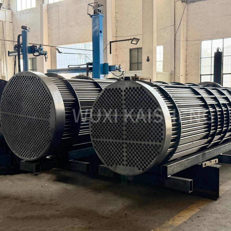
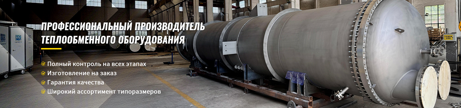
Выбор материалов и соблюдение стандартов — это сфера, где опыт производителя играет решающую роль. CompanyWuxi Kaisheng Electric Power and Petrochemical Equipment Co., Ltd.специализируется именно на разработке и производстве высококачественного теплообменного оборудования для сложных условий эксплуатации. Наш ассортимент включает титановые кожухотрубные теплообменники, незаменимые для опреснения морской воды и агрессивных сред, а также аппараты высокого давления, сертифицированные по стандартам ASME и PED. Мы производим трубные пучки из различных материалов: гофрированные из нержавеющей стали 316, морскую латунь C46400, медно-никелевые сплавы и никелевые сплавы N06625, обеспечивая высокую коррозионную стойкость и теплоэффективность. Наша продукция, включая воздушные охладители и котлы-утилизаторы, широко применяется в нефтепереработке, химической промышленности, судостроении и энергетике по всему миру. Мы понимаем, что экономия на металле или упрощение технологии сварки ради снижения цены недопустима, когда речь идет об оборудовании, работающем под давлением и температурой, поэтому каждый наш проект проходит строгий контроль качества.

Frequently Asked Questions

Как часто нужно чистить кожухотрубный теплообменник?

Периодичность чистки зависит исключительно от качества теплоносителей и заложенного запаса по загрязнению. Для систем с подготовленной водой (умягченной, деаэрированной) межремонтный интервал может достигать 2-3 лет. Для систем с речной или оборотной водой чистка может требоваться каждые 6-12 месяцев. Индикатором необходимости чистки служит рост температуры на выходе нагреваемой среды при неизменных расходах или рост перепада давления. Мы рекомендуем вести журнал температурных режимов, чтобы отслеживать тенденцию ухудшения теплопередачи.

Можно ли увеличить мощность существующего теплообменника без его замены?

Да, в некоторых случаях это возможно. Основные методы: увеличение скорости потока (если позволяет запас давления насосов), улучшение качества воды (снижение загрязнения), замена трубного пучка на более эффективный (например, с трубами меньшего диаметра или оребренными), либо изменение схемы движения (увеличение числа ходов). Однако радикально увеличить мощность (более чем на 20-30%) без замены корпуса обычно не удается. Часто проще и дешевле установить второй теплообменник параллельно первому.

Какой материал труб лучше выбрать для морской воды?

Для морской воды обычная углеродистая сталь непригодна из-за высокой коррозии. Медно-никелевые сплавы (например, мельхиор) традиционно использовались для этих целей, но они дороги. Современным и наиболее надежным решением является титан. Титановые трубы абсолютно стойки к морской воде, имеют высокий коэффициент теплоотдачи и долгий срок службы. Несмотря на высокую начальную стоимость, титановые теплообменники часто оказываются выгоднее в долгосрочной перспективе благодаря отсутствию простоев на ремонт и замену. Именно такие решения мы активно внедряем в проектах по опреснению и морской энергетике.

В чем разница между одноходовым и многоходовым теплообменником?

В одноходовом аппарате теплоноситель проходит через все трубы от одной крышки к другой за один раз. Это обеспечивает минимальное гидравлическое сопротивление, но низкую скорость потока при большом количестве труб. В многоходовом аппарате поток делится на несколько последовательных частей, проходя через часть труб, разворачиваясь в камере и проходя через другую Part. Это позволяет увеличить скорость потока в 2, 4, 6 и более раз, существенно повысив коэффициент теплоотдачи, но ценой роста перепада давления и усложнения конструкции (наличие продольных перегородок в камерах).

Заключение и рекомендации к действию

Расчет теплопередачи кожухотрубного теплообменника — это сложный инженерный процесс, требующий учета множества взаимозависимых факторов: от физико-химических свойств сред до гидравлических характеристик насосов и требований стандартов безопасности. Ошибки на этапе проектирования стоят дорого: либо в виде неэффективной работы системы и перерасхода энергии, либо в виде аварийных ситуаций и внеплановых остановок.

Мы убедились на собственном опыте, что универсальных решений не существует. Каждый технологический процесс уникален. Использование упрощенных методов или копирование проектов без адаптации к местным условиям — путь к проблемам. Грамотный расчет требует профессионализма, актуальных данных и соблюдения нормативной базы.

Если вы планируете модернизацию системы теплоснабжения, внедрение нового технологического процесса или замену устаревшего оборудования, не рискуйте, полагаясь на приблизительные оценки. Доверьте расчет и подбор оборудования профессионалам, которые несут ответственность за результат.

Contact us todayдля получения консультации по вашему проекту. Инженеры компании ООО «Уси Кайшэн» готовы провести детальныйрасчет кожухотрубного теплообменникас учетом всех ваших требований, подготовить технико-коммерческое предложение и обеспечить поставку сертифицированного оборудования (ASME, PED), которое прослужит десятилетия в самых суровых условиях эксплуатации.